Is the Beta Distribution a Member of the Location-scale Family
5.17: The Beta Distribution
- Folio ID
- 10357

\(\newcommand{\R}{\mathbb{R}}\) \(\newcommand{\N}{\mathbb{Northward}}\) \(\newcommand{\Eastward}{\mathbb{Due east}}\) \(\newcommand{\P}{\mathbb{P}}\) \(\newcommand{\var}{\text{var}}\) \(\newcommand{\sd}{\text{sd}}\) \(\newcommand{\cov}{\text{cov}}\) \(\newcommand{\cor}{\text{cor}}\) \(\newcommand{\skw}{\text{skew}}\) \(\newcommand{\kur}{\text{kurt}}\)
In this section, nosotros will written report the beta distribution, the most of import distribution that has divisional support. Merely before we can study the beta distribution we must study the beta function.
The Beta Function
Definition
The beta role \( B \) is defined as follows: \[ B(a, b) = \int_0^1 u^{a-one} (1 - u)^{b - 1} du; \quad a, \, b \in (0, \infty) \]
Proof that \( B \) is well divers
We need to show that \(B(a, b) \lt \infty\) for every \(a, \, b \in (0, \infty)\). The integrand is positive on \( (0, 1) \), so the integral exists, either as a real number or \( \infty \). If \( a \ge ane \) and \( b \ge one \), the integrand is continuous on \( [0, ane] \), so of course the integral is finite. Thus, the only cases of interest are when \( 0 \lt a \lt one \) or \( 0 \lt b \lt 1 \). Note that \[ \int_0^1 u^{a-ane} (i - u)^{b - 1} du = \int_0^{one/two} u^{a-1} (i - u)^{b - 1} du + \int_{one/2}^i u^{a-1} (i - u)^{b - 1} du \] If \(0 \lt a \lt ane\), \((1 - u)^{b-1}\) is divisional on \(\left(0, \frac{1}{two}\correct]\) and \( \int_0^{1/2} u^{a - 1} \, du = \frac{1}{a 2^a} \). Hence the kickoff integral on the right in the displayed equation is finite. Similarly, If \(0 \lt b \lt 1\), \(u^{a-i}\) is divisional on \(\left[\frac{1}{2}, i\correct)\) and \( \int_{one/2}^ane (1 - u)^{b-1} \, du = \frac{1}{b ii^b} \). Hence the 2d integral on the correct in the displayed equation is as well finite.
The beta office was first introduced by Leonhard Euler.
Backdrop
The beta function satisfies the post-obit properties:
- \(B(a, b) = B(b, a)\) for \( a, \, b \in (0, \infty) \), so \( B \) is symmetric.
- \(B(a, i) = \frac{1}{a}\) for \( a \in (0, \infty) \)
- \( B(1, b) = \frac{i}{b} \) for \( b \in (0, \infty) \)
Proof
- Using the commutation \( 5 = 1 - u \) we have \[ B(a, b) = \int_0^ane u^{a-i}(i - u)^{b-1} du = \int_0^1 (1 - five)^{a-1} v^{b-1} dv = B(b, a) \]
- \( B(a, i) = \int_0^1 u^{a-1} du = \frac{1}{a} \)
- This follows from (a) and (b).
The beta role has a simple expression in terms of the gamma part:
If \( a, \, b \in (0, \infty) \) then \[ B(a, b) = \frac{\Gamma(a) \Gamma(b)}{\Gamma(a + b)} \]
Proof
From the definitions, nosotros can limited \(\Gamma(a + b) B(a, b)\) as a double integral: \[ \Gamma(a + b) B(a, b) = \int_0^\infty x^{a + b -1} eastward^{-x} dx \int_0^1 y^{a-1} (1 - y)^{b-1} dy = \int_0^\infty \int_0^i (x y)^{a-ane}[10 (1 - y)]^{b-1} 10 e^{-x} dx \, dy \] Side by side nosotros use the transformation \(w = x y\), \(z = x (1 - y)\) which maps \((0, \infty) \times (0, 1) \) one-to-ane onto \( (0, \infty) \times (0, \infty) \). The inverse transformation is \( x = w + z \), \( y = w \large/(w + z) \) and the absolute value of the Jacobian is \[ \left|\det\frac{\fractional(x, y)}{\partial(westward, z)}\right| = \frac{ane}{(due west + z)} \] Thus, using the change of variables theorem for multiple integrals, the integral above becomes \[ \int_0^\infty \int_0^\infty west^{a-i} z^{b-1} (w + z) due east^{-(w + z)} \frac{1}{w + z} dw \, dz \] which after simplifying is \( \Gamma(a) \Gamma(b) \).
Recall that the gamma function is a generalization of the factorial office. Here is the corresponding result for the beta office:
If \(j, \, m \in \N_+\) then \[ B(j, k) = \frac{(j - 1)! (k - ane)!}{(j + k - ane)!} \]
Proof
Call back that \( \Gamma(north) = (n - 1)! \) for \( north \in \N_+ \), so this result follows from the previous one.
Allow's generalize this result. First, call up from our written report of combinatorial structures that for \(a \in \R\) and \(j \in \Northward\), the ascending power of base \( a \) and order \( j \) is \[ a^{[j]} = a (a + one) \cdots [a + (j - one)] \]
If \(a, \, b \in (0, \infty)\), and \(j, \, k \in \N\), then \[ \frac{B(a + j, b + k)}{B(a, b)} = \frac{a^{[j]} b^{[k]}}{(a + b)^{[j + thou]}} \]
Proof
Recall that \( \Gamma(a + j) = a^{[j]} \Gamma(a) \), and so the result follows from the representation to a higher place for the beta office in terms of the gamma function.
\(B\left(\frac{i}{2}, \frac{one}{two}\right) = \pi\).
Proof
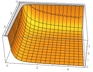
Figure \(\PageIndex{1}\): The graph of \(B(a, b)\) on the square \(0 \lt a \lt five\), \(0 \lt b \lt v\)
The Incomplete Beta Role
The integral that defines the beta function can be generalized by changing the interval of integration from \((0, i)\) to \((0, x)\) where \(ten \in [0, one]\).
The incomplete beta function is defined as follows \[ B(x; a, b) = \int_0^x u^{a-1} (1 - u)^{b-1} du, \quad x \in (0, 1); \; a, \, b \in (0, \infty) \]
Of course, the ordinary (complete) beta function is \(B(a, b) = B(i; a, b)\) for \( a, \, b \in (0, \infty) \).
The Standard Beta Distribution
Distribution Functions
The beta distributions are a family of continuous distributions on the interval \( (0, 1) \).
The (standard) beta distribution with left parameter \( a \in (0, \infty) \) and right parameter \( b \in (0, \infty) \) has probability density function \( f \) given past \[ f(x) = \frac{1}{B(a, b)} x^{a-1} (1 - 10)^{b-1}, \quad x \in (0, ane) \]
Of grade, the beta function is simply the normalizing constant, so it's clear that \( f \) is a valid probability density function. If \( a \ge 1 \), \( f \) is divers at 0, and if \( b \ge 1 \), \( f \) is defined at 1. In these cases, it's customary to extend the domain of \( f \) to these endpoints. The beta distribution is useful for modeling random probabilities and proportions, especially in the context of Bayesian analysis. The distribution has only two parameters and yet a rich diverseness of shapes (so in particular, both parameters are shape parameters). Qualitatively, the kickoff order properties of \( f \) depend on whether each parameter is less than, equal to, or greater than 1.
For \( a, \, b \in (0, \infty) \) with \( a + b \ne 2 \), define \[ x_0 = \frac{a - ane}{a + b - two} \]
- If \(0 \lt a \lt 1\) and \(0 \lt b \lt 1\), \( f \) decreases and so increases with minimum value at \(x_0 \) and with \( f(x) \to \infty \) as \( x \downarrow 0 \) and as \( ten \uparrow one \).
- If \(a = 1\) and \(b = one\), \( f \) is constant.
- If \(0 \lt a \lt 1\) and \(b \ge ane\), \( f \) is decreasing with \( f(x) \to \infty \) as \( x \downarrow 0 \).
- If \(a \ge one\) and \(0 \lt b \lt i\), \( f \) is increasing with \( f(x) \to \infty \) as \( x \uparrow 1 \).
- If \(a = 1\) and \(b \gt 1\), \( f \) is decreasing with mode at \( x = 0 \).
- If \(a \gt one\) and \(b = 1\), \( f \) is increasing with mode at \( 10 = 1 \).
- If \(a \gt one\) and \(b \gt 1\), \( f \) increases and and so decreases with mode at \( x_0 \).
Proof
These results follow from standard calculus. The commencement derivative is \[ f^\prime(x) = \frac{1}{B(a, b)} x^{a - 2}(one - ten)^{b - 2} [(a - 1) - (a + b - 2) x], \quad 0 \lt 10 \lt i \]
From role (b), note that the special case \(a = i\) and \(b = 1\) gives the continuous compatible distribution on the interval \((0, 1)\) (the standard uniform distribution). Note also that when \(a \lt 1\) or \(b \lt 1\), the probability density function is unbounded, and hence the distribution has no way. On the other hand, if \(a \ge one\), \(b \ge 1\), and 1 of the inequalites is strict, the distribution has a unique way at \( x_0 \). The second order properties are more than complicated.
For \( a, \, b \in (0, \infty) \) with \( a + b \notin \{two, 3\} \) and \( (a - 1)(b - 1)(a + b - 3) \ge 0 \), define \brainstorm{align} x_1 &= \frac{(a - 1)(a + b - iii) - \sqrt{(a - one)(b - 1)(a + b - 3)}}{(a + b - iii)(a + b - 2)}\\ x_2 &= \frac{(a - i)(a + b - 3) + \sqrt{(a - 1)(b - 1)(a + b - 3)}}{(a + b - 3)(a + b - 2)} \end{marshal} For \( a \lt i \) and \( a + b = 2 \) or for \( b \lt 1 \) and \( a + b = 2 \), define \( x_1 = x_2 = 1 - a / 2 \).
- If \( a \le one \) and \( b \le 1 \), or if \( a \le 1 \) and \( b \ge 2 \), or if \( a \ge 2 \) and \( b \le 1 \), \( f \) is concave upward.
- If \( a \le ane \) and \( 1 \lt b \lt 2 \), \( f \) is concave upwardly so downwards with inflection point at \( x_1 \).
- If \( ane \lt a \lt 2 \) and \( b \le one \), \( f \) is concave downwards and and then upward with inflection point at \( x_2 \).
- If \( 1 \lt a \le 2 \) and \( 1 \lt b \le ii \), \( f \) is concave downwardly.
- If \( one \lt a \le 2 \) and \( b \gt 2 \), \( f \) is concave downward then upward with inflection point at \( x_2 \).
- If \( a \gt 2 \) and \( ane \lt b \le two \), \( f \) is concave upwardly and and then downwards with inflection signal at \( x_1 \).
- If \( a \gt ii \) and \( b \gt 2 \), \( f \) is concave upward, then downwards, then upward again, with inflection points at \( x_1 \) and \( x_2 \).
Proof
These results follow from standard (but very tedious) calculus. The 2nd derivative is \[ f^{\prime\prime number}(x) = \frac{1}{B(a, b)} 10^{a - 3}(one - ten)^{b - 3} \left[(a + b - two)(a + b - 3) x^2 - two (a - 1)(a + b - 3) x + (a - 1)(a - 2)\correct] \]
In the special distribution simulator, select the beta distribution. Vary the parameters and note the shape of the beta density office. For selected values of the parameters, run the simulation 1000 times and compare the empirical density function to the true density function.
The special case \(a = \frac{i}{2}\), \(b = \frac{i}{2}\) is the arcsine distribution, with probability density function given past \[ f(10) = \frac{1}{\pi \, \sqrt{x (1 - x)}}, \quad x \in (0, 1) \] This distribution is important in a number of applications, and so the arcsine distribution is studied in a separate section.
The beta distribution function \(F\) can be easily expressed in terms of the incomplete beta function. Equally usual \(a\) denotes the left parameter and \(b\) the correct parameter.
The beta distribution function \( F \) with parameters \(a, \, b \in (0, \infty)\) is given by \[ F(x) = \frac{B(x; a, b)}{B(a, b)}, \quad ten \in (0, 1) \]
The distribution function \( F \) is sometimes known as the regularized incomplete beta part. In some special cases, the distribution role \(F\) and its inverse, the quantile function \(F^{-1}\), can be computed in closed form, without resorting to special functions.
If \(a \in (0, \infty)\) and \(b = 1\) and then
- \(F(x) = 10^a\) for \(ten \in (0, one)\)
- \(F^{-1}(p) = p^{1/a}\) for \(p \in (0, 1)\)
If \(a = 1\) and \(b \in (0, \infty)\) then
- \(F(x) = 1 - (1 - x)^b\) for \(ten \in (0, 1)\)
- \(F^{-1}(p) = one - (1 - p)^{1/b}\) for \(p \in (0, 1)\)
If \(a = b = \frac{1}{2}\) (the arcsine distribution) and so
- \(F(x) = \frac{2}{\pi} \arcsin\left(\sqrt{x}\right)\) for \(x \in (0, 1)\)
- \(F^{-1}(p) = \sin^ii\left(\frac{\pi}{two} p\right)\) for \(p \in (0, 1)\)
At that place is an interesting relationship between the distribution functions of the beta distribution and the binomial distribution, when the beta parameters are positive integers. To state the human relationship we need to embellish our notation to indicate the dependence on the parameters. Thus, let \(F_{a, b}\) denote the beta distribution function with left parameter \(a \in (0, \infty)\) and right parameter \(b \in (0, \infty)\), and let \(G_{north,p}\) denote the binomial distribution function with trial parameter \(n \in \N_+\) and success parameter \(p \in (0, ane)\).
If \(j, \, k \in \N_+\) and \(x \in (0, i)\) then \[ F_{j,thou}(x) = G_{j + one thousand - one, ane - x}(thou - 1) \]
Proof
By definition \[ F_{j,k}(x) = \frac{i}{B(j,thousand)} \int_0^x t^{j-1} (1 - t)^{k-1} dt \] Integrate by parts with \( u = (1 - t)^{g-1} \) and \( dv = t^{j-1} dt \), so that \( du = -(k -1) (i - t)^{k-2} \) and \( v = t^j / j \). The issue is \[ F_{j,k}(ten) = \frac{1}{j B(j, chiliad)} (1 - 10)^{1000-one} x^j + \frac{k-1}{j B(j, k)} \int_0^10 t^j (1 - t)^{grand-2} dt\] Simply by the holding of the beta part to a higher place, \( B(j, thousand) = (j - one)! (k - 1)! \large/(j + k - 1)! \). Hence \( 1 \big/ j B(j, k) = \binom{j + k - 1}{thousand - 1} \) and \( (k - 1) \big/ j B(j, thou) = i \big/ B(j + 1, chiliad - ane) \). Thus, the last displayed equation can be rewritten every bit \[F_{j,k}(x) = \binom{j + k - 1}{one thousand - 1} (one - x)^{k-1} ten^j + F_{j + i, grand - 1}(10)\] Recall from the special case above that \(F_{j + k - ane, 1}(x) = x^{j + one thousand - 1}\). Iterating the terminal displayed equation gives the result.
In the special distribution figurer, select the beta distribution. Vary the parameters and annotation the shape of the density part and the distribution function. In each of the following cases, notice the median, the starting time and third quartiles, and the interquartile range. Sketch the boxplot.
- \(a = 1\), \(b = 1\)
- \(a = 1\), \(b = 3\)
- \(a = three\), \(b = 1\)
- \(a = 2\), \(b = 4\)
- \(a = 4\), \(b = 2\)
- \(a = iv\), \(b = 4\)
Moments
The moments of the beta distribution are like shooting fish in a barrel to express in terms of the beta office. As before, suppose that \(X\) has the beta distribution with left parameter \(a \in (0, \infty)\) and right parameter \(b \in (0, \infty)\).
If \(k \in [0, \infty)\) then \[ \E\left(X^k\right) = \frac{B(a + k, b)}{B(a, b)} \] In particular, if \( k \in \N \) so \[ \E\left(Ten^grand\correct) = \frac{a^{[grand]}}{(a + b)^{[k]}} \]
Proof
Note that \[ \E\left(X^m\right) = \int_0^1 10^k \frac{ane}{B(a, b)} x^{a-1} (1 - 10)^{b - 1} dx = \frac{ane}{B(a, b)} \int_0^1 x^{a + yard - 1} (ane - ten)^{b - one} dx = \frac{B(a + k, b)}{B(a, b)}\] If \( k \in \N \), the formula simplifies by the belongings of the beta function to a higher place.
From the full general formula for the moments, it'south straightforward to compute the mean, variance, skewness, and kurtosis.
The mean and variance of \( Ten \) are \begin{align} \Due east(Ten) &= \frac{a}{a + b} \\ \var(X) &= \frac{a b}{(a + b)^2 (a + b + i)} \end{marshal}
Proof
The formula for the mean and variance follow from the formula for the moments and the computational formula \( \var(X) = \East(X^2) - [\East(X)]^2 \)
Note that the variance depends on the parameters \( a \) and \( b \) only through the production \( a b \) and the sum \( a + b \).
Open the special distribution simulator and select the beta distribution. Vary the parameters and note the size and location of the mean\(\pm\)standard difference bar. For selected values of the parameters, run the simulation m times and compare the sample mean and standard departure to the distribution mean and standard deviation.
The skewness and kurtosis of \( X \) are \begin{align} \skw(X) &= \frac{two (b - a) \sqrt{a + b + 1}}{(a + b + 2) \sqrt{a b}} \\ \kur(X) &= \frac{three a^iii b + 3 a b^3 + half-dozen a^2 b^two + a^iii + b^iii + thirteen a^2 b + 13 a b^2 + a^ii + b^2 + 14 a b}{a b (a + b + two) (a + b + 3)} \terminate{align}
Proof
These results follow from the computational formulas that requite the skewness and kurtosis in terms of \( \East(X^k) \) for \( k \in \{1, 2, iii, 4\} \), and the formula for the moments above.
In particular, note that the distribution is positively skewed if \( a \lt b \), unskewed if \( a = b \) (the distribution is symmetric about \( x = \frac{1}{ii} \) in this case) and negatively skewed if \( a \gt b \).
Open the special distribution simulator and select the beta distribution. Vary the parameters and annotation the shape of the probability density part in light of the previous result on skewness. For various values of the parameters, run the simulation thousand times and compare the empirical density office to the true probability density part.
Related Distributions
The beta distribution is related to a number of other special distributions.
If \(10\) has the beta distribution with left parameter \(a \in (0, \infty)\) and right parameter \(b \in (0, \infty)\) so \(Y = 1 - Ten\) has the beta distribution with left parameter \(b\) and right parameter \(a\).
Proof
This follows from the standard change of variables formula. If \( f \) and \( thou \) denote the PDFs of \( X \) and \( Y \) respectively, then \[ g(y) = f(1 - y) = \frac{i}{B(a, b)} (ane - y)^{a - ane} y^{b - one} = \frac{1}{B(b, a)} y^{b - 1} (i - y)^{a - ane}, \quad y \in (0, 1)\]
The beta distribution with right parameter 1 has a reciprocal relationship with the Pareto distribution.
Suppose that \( a \in (0, \infty) \).
- If \(X\) has the beta distribution with left parameter \(a \) and right parameter i then \(Y = 1 / X\) has the Pareto distribution with shape parameter \(a\).
- If \( Y \) has the Pareto distribution with shape parameter \( a \) then \( X = 1 / Y \) has the beta distribution with left parameter \( a \) and right parameter 1.
Proof
The ii results are equivalent. In (a), suppose that \( X \) has the beta distribution with parameters \( a \) and 1. The transformation \( y = 1 / x \) maps \( (0, 1) \) 1-to-one onto \( (0, \infty) \). The changed is \( x = 1 / y \) with \( dx/dy = -1/y^2 \). Recall also that \( B(a, 1) = i / a \). By the change of variables formula, the PDF \( g \) of \( Y = 1 / 10 \) is given by \[ g(y) = f\left(\frac{1}{y}\right) \frac{1}{y^ii} = a \left(\frac{1}{y}\right)^{a-ane} \frac{ane}{y^2} = \frac{a}{y^{a+1}}, \quad y \in (0, \infty) \] We recognize \( g \) every bit the PDF of the Pareto distribution with shape parameter \( a \).
The following result gives a connection between the beta distribution and the gamma distribution.
Suppose that \(X\) has the gamma distribution with shape parameter \(a \in (0, \infty)\) and rate parameter \(r \in (0, \infty)\), \(Y\) has the gamma distribution with shape parameter \(b \in (0, \infty)\) and rate parameter \(r\), and that \(Ten\) and \(Y\) are contained. Then \(5 = X \big/ (X + Y)\) has the beta distribution with left parameter \(a\) and right parameter \(b\).
Proof
Let \( U = 10 + Y \) and \( Five = X \large/ (X + Y) \). We volition actually prove stronger results: \( U \) and \( V \) are independent, \( U \) has the gamma distribution with shape parameter \( a + b \) and rate parameter \( r \), and \( Five \) has the beta distribution with parameters \( a \) and \( b \). First note that \( (Ten, Y) \) has joint PDF \( f \) given by \[ f(x, y) = \frac{r^a}{\Gamma(a)} 10^{a-1} due east^{-r x} \frac{r^b}{\Gamma(b)} y^{b-1} e^{-r y} = \frac{r^{a+b}}{\Gamma(a) \Gamma(b)} ten^{a-1} y^{b-1} e^{-r(ten + y)}; \quad x, \, y \in (0, \infty) \] The transformation \( u = x + y \) and \( v = x \big/ (x + y) \) maps \( (0, \infty) \times (0, \infty) \) one-to-1 onto \( (0, \infty) \times (0, 1) \). The inverse is \( x = u v \), \( y = u(1 - 5) \) and the absolute value of the Jacobian is \[ \left|\det \frac{\partial(10, y)}{\partial(u, v)}\right| = u \] Hence past the multivariate change of variables theorem, the PDF \( g \) of \( (U, V) \) is given past \begin{marshal} g(u, 5) & = f[u v, u(1 - v)] u = \frac{r^{a+b}}{\Gamma(a) \Gamma(b)} (u v)^{a-1} [u(1 - v)]^{b-ane} e^{-ru} u \\ & = \frac{r^{a+b}}{\Gamma(a) \Gamma(b)} u^{a+b-1} e^{-ru} five^{a-1} (1 - five)^{b-1} \\ & = \frac{r^{a+b}}{\Gamma(a + b)} u^{a+b-1} e^{-ru} \frac{\Gamma(a + b)}{\Gamma(a) \Gamma(b)} 5^{a-1} (1 - v)^{b-ane}; \quad u \in (0, \infty), five \in (0, i) \finish{marshal} The results now follow from the factorization theorem. The factor in \( u \) is the gamma PDF with shape parameter \( a + b \) and rate parameter \( r \) while the factor in \( 5 \) is the beta PDF with parameters \( a \) and \( b \).
The post-obit result gives a connectedness betwixt the beta distribution and the \(F\) distribution. This connexion is a minor variation of the previous result.
If \(X\) has the \(F\) distribution with \(n \in (0, \infty)\) degrees of freedom in the numerator and \(d \in (0, \infty)\) degrees of freedom in the denominator then \[ Y = \frac{(due north / d) X}{1 + (due north / d)Ten} \] has the beta distribution with left parameter \(a = due north / 2\) and correct parameter \(b = d / two\).
Proof
If \(X\) has the \(F\) distribution with \(n \gt 0\) degrees of liberty in the numerator and \(d \gt 0\) degrees of freedom in the denominator and so \( X \) can be written as \[ X = \frac{U / n}{V / d} \] where \( U \) has the chi-square distribution with \( n \) degrees of freedom, \( V \) has the chi-foursquare distribution with \( d \) degrees of freedom, and \( U \) and \( V \) are contained. Hence \[ Y = \frac{(n / d) X}{1 + (northward / d) X} = \frac{U / V}{1 + U / V} = \frac{U}{U + V} \] Only the chi-foursquare distribution is a special case of the gamma distribution. Specifically, \( U \) has the gamma distribution with shape parameter \( n / 2 \) and charge per unit parameter \( 1/2 \), \( V \) has the gamma distribution with shape parameter \( d / two \) and rate parameter \( 1/two \), and again \( U \) and \( V \) are independent. Hence by the previous result, \( Y \) has the beta distribution with left parameter \( north/2 \) and right parameter \( d/two \).
Our adjacent result is that the beta distribution is a fellow member of the general exponential family of distributions.
Suppose that \(X\) has the beta distribution with left parameter \(a \in (0, \infty)\) and right parameter \(b \in (0, \infty)\). And so the distribution is a two-parameter exponential family with natural parameters \(a - 1\) and \(b - 1\), and natural statistics \(\ln(10)\) and \(\ln(one - X)\).
Proof
This follows from the definition of the general exponential distribution, since the PDF \( f \) of \( X \) can be written equally \[ f(10) = \frac{i}{B(a, b)} \exp\left[(a - i) \ln(x) + (b - one) \ln(ane - ten)\correct], \quad x \in (0, i) \]
The beta distribution is too the distribution of the order statistics of a random sample from the standard uniform distribution.
Suppose \( north \in \N_+ \) and that \( (X_1, X_2, \ldots, X_n) \) is a sequence of contained variables, each with the standard compatible distribution. For \( chiliad \in \{1, 2, \ldots, n\} \), the \( k \)th order statistics \( X_{(k)} \) has the beta distribution with left parameter \( a = thou \) and correct parameter \( b = n - k + ane \).
Proof
See the section on society statistics.
1 of the most important properties of the beta distribution, and one of the main reasons for its wide apply in statistics, is that it forms a conjugate family for the success probability in the binomial and negative binomial distributions.
Suppose that \( P \) is a random probability having the beta distribution with left parameter \( a \in (0, \infty) \) and correct parameter \( b \in (0, \infty) \). Suppose as well that \( X \) is a random variable such that the provisional distribution of \( X \) given \( P = p \in (0, i) \) is binomial with trial parameter \( n \in \N_+ \) and success parameter \( p \). Then the conditional distribution of \( P \) given \( 10 = 1000 \) is beta with left parameter \( a + k \) and correct parameter \( b + north - k \).
Proof
The joint PDF \( f \) of \( (P, X) \) on \( (0, 1) \times \{0, one, \ldots n\} \) is given by \[ f(p, 1000) = \frac{one}{B(a, b)} p^{a-1} (1 - p)^{b-1} \binom{due north}{thousand} p^k (1 - p)^{northward-thou} = \frac{1}{B(a, b)} \binom{n}{thousand} p^{a + grand - 1} (i - p)^{b + n - k - 1} \] The conditional PDF of \( P \) given \( X = thousand \) is merely the normalized version of the role \( p \mapsto f(p, one thousand) \). Nosotros can tell from the functional form that this distribution is beta with the parameters given in the theorem.
Suppose again that \( P \) is a random probability having the beta distribution with left parameter \( a \in (0, \infty) \) and right parameter \( b \in (0, \infty) \). Suppose as well that \( North \) is a random variable such that the conditional distribution of \( N \) given \( P = p \in (0, 1) \) is negative binomial with stopping parameter \( k \in \N_+ \) and success parameter \( p \). Then the conditional distribution of \( P \) given \( Due north = n \) is beta with left parameter \( a + 1000 \) and right parameter \( b + northward - k \).
Proof
The joint PDF \( f \) of \( (P, N) \) on \( (0, one) \times \{m, 1000 + 1, \ldots\} \) is given by \[ f(p, north) = \frac{1}{B(a, b)} p^{a-1} (1 - p)^{b-1} \binom{north - 1}{yard - 1} p^k (1 - p)^{n-g} = \frac{1}{B(a, b)} \binom{due north - one}{1000 - i} p^{a + m - 1} (1 - p)^{b + north - chiliad - i} \] The conditional PDF of \( P \) given \( N = due north \) is simply the normalized version of the office \( p \mapsto f(p, n) \). We can tell from the functional form that this distribution is beta with the parameters given in the theorem.
in both cases, notation that in the posterior distribution of \( P \), the left parameter is increased past the number of successes and the right parameter by the number of failures. For more on this, run across the section on Bayesian interpretation in the affiliate on betoken estimation.
The Full general Beta Distribution
The beta distribution tin can be hands generalized from the support interval \((0, i)\) to an arbitrary bounded interval using a linear transformation. Thus, this generalization is merely the location-scale family associated with the standard beta distribution.
Suppose that \(Z\) has the standard beta distibution with left parameter \(a \in (0, \infty)\) and correct parameter \(b \in (0, \infty)\). For \(c \in \R\) and \(d \in (0, \infty)\) random variable \(10 = c + d Z\) has the beta distribution with left parameter \( a \), right parameter \( b \), location parameter \( c \) and scale parameter \( d \).
For the remainder of this discussion, suppose that \( X \) has the distribution in the definition above.
\(Ten\) has probability density function
\[ f(x) = \frac{1}{B(a, b) d^{a + b - 1}} (x - c)^{a - i} (c + d - x)^{b - i}, \quad x \in (c, c + d) \]
Proof
This follows from a standard event for location-calibration families. If \( g \) denotes the standard beta PDF of \( Z \), then \( Ten \) has PDF \( f \) given by \[ f(x) = \frac{1}{d} thousand\left(\frac{10 - c}{d}\correct), \quad x \in (c, c + d) \]
Nigh of the results in the previous sections accept simple extensions to the full general beta distribution.
The mean and variance of \( Ten \) are
- \(\E(X) = c + d \frac{a}{a + b}\)
- \(\var(X) = d^2 \frac{a b}{(a + b)^two (a + b + one)}\)
Proof
This follows from the standard mean and variance and bones backdrop of expected value and variance.
- \( \East(Ten) = c + d \E(Z)\)
- \( \var(10) = d^2 \var(Z) \)
Call up that skewness and variance are defined in terms of standard scores, and hence are unchanged under location-scale transformations. Hence the skewness and kurtosis of \( X \) are just as for the standard beta distribution.
Source: https://stats.libretexts.org/Bookshelves/Probability_Theory/Book%3A_Probability_Mathematical_Statistics_and_Stochastic_Processes_(Siegrist)/05%3A_Special_Distributions/5.17%3A_The_Beta_Distribution
Post a Comment for "Is the Beta Distribution a Member of the Location-scale Family"